Sometimes in Excel you might want to find the maximum or minimum value for subcategories within a dataset.
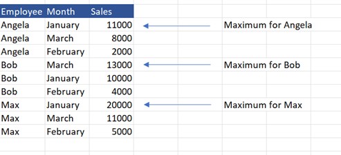
For example, say my dataset looked like this:
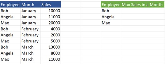
How can we write a formula to populate the “Max Sales in a Month” column in the final green table?
Built-in Functions – Excel 2021
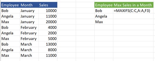
If you are using later versions of Excel (2021, Office 365), Microsoft has incorporated MAXIFS and MINIFS as standard functions. These can easily accomplish the task:
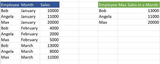
Final result:
Array Formulas
You can also use arrays. However, arrays can slow down your workbook and may be difficult for others in the organization to use.
Using MAXIFS or MINIFS without Arrays
Have no fear, you can replicate MAXIFS and MINIFS without arrays by sorting your data and using formulas.
Writing a MAXIFS or MINIFS formula without arrays will ultimately require two steps:
- Sort the dataset by employee and then by sales, choosing “Largest to Smallest” for the sales column for a MAXIFS and “Smallest to Largest” for a MINIFS
- Use a VLOOKUP to grab the first value for each employee and populate the final table
Sort the Data to Assist Your Formula
Though this solution requires one manual step, first sort your data by subcategory and then by the numeric value you wish to find the maximum or minimum of for each subcategory. In this example, the subcategory is “Employee,” and the numeric value is “Sales.”
Because we want to find the maximum sales in one month by each employee, we will choose the “Largest to Smallest” option for the Sales column.
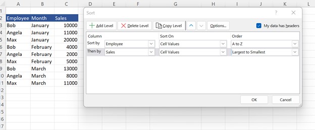
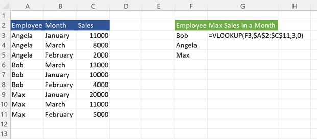
Once we’ve sorted the values by Employee and Sales (largest to smallest), all the maximum values for each employee have moved to the first row that employee’s name appears in the table:
Use a VLOOKUP to Populate the Final Maximum or Minimum Table
Now we can use a VLOOKUP to populate the final green table. Using the employee name as our lookup value, the VLOOKUP returns the corresponding sales value for the first time each employee name appears in the “Employee” column.
Because we sorted the data first, the VLOOKUP will return the maximum sales value for each employee:
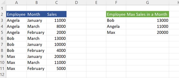
And there you have it!
Though this method requires the user to sort the data manually, it can save a significant amount of time and formulas compared to arrays, especially for large datasets.