If you’re looking to unpivot data in Excel using formulas, you might be in one of two situations:
Situation 1: You just want to delete or reformat your pivot. If that’s your situation, please see this article from Microsoft.
Situation 2: You want to take multiple columns of a dataset and collapse them into a single column, which is the equivalent of the melt function in R or pandas. This article addresses this problem.
Tidy data and situations where it helps to unpivot data in Excel using formulas
Although other ways of displaying data might be visually more pleasing, it can be advantageous to present data in a tidy format, where each row of data can have multiple variables, but only a single value.
Generally, I find tidy data is much easier to analyze or necessary to upload data back into a database or pass along for more official analysis.
Unfortunately, Excel doesn’t have a single function or easy way to reformat a dataset into a tidy format, like R or the pandas library in Python. And if you’re trying to keep things within Excel so your coworkers don’t have to use those other languages, it can be a real challenge.
How to unpivot data in excel using formulas
Luckily, if you need to have your spreadsheet consistently reformat data in a tidy format as part of a repetitive process, you can “unpivot” data in Excel just using formulas. Please note, this method can be resource intensive if the dataset is too large.
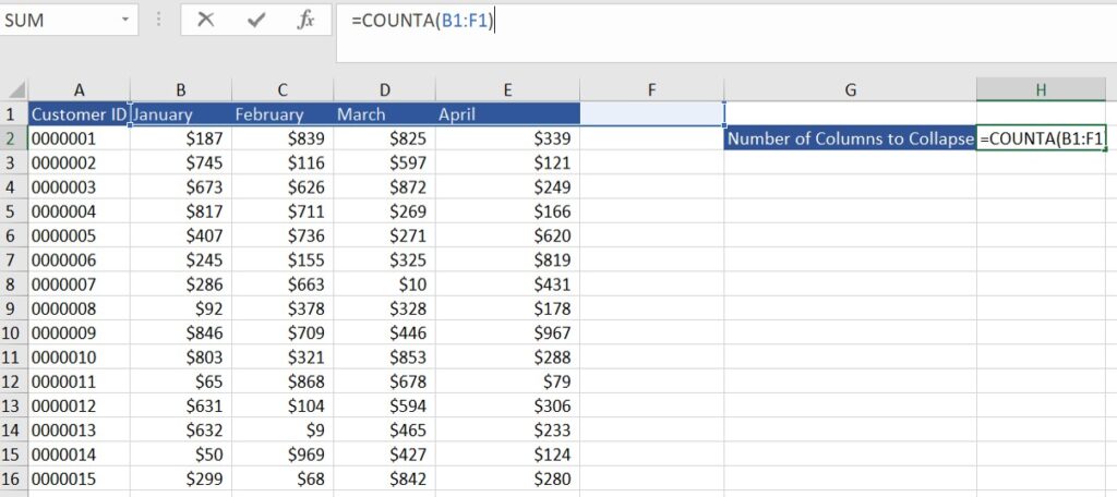
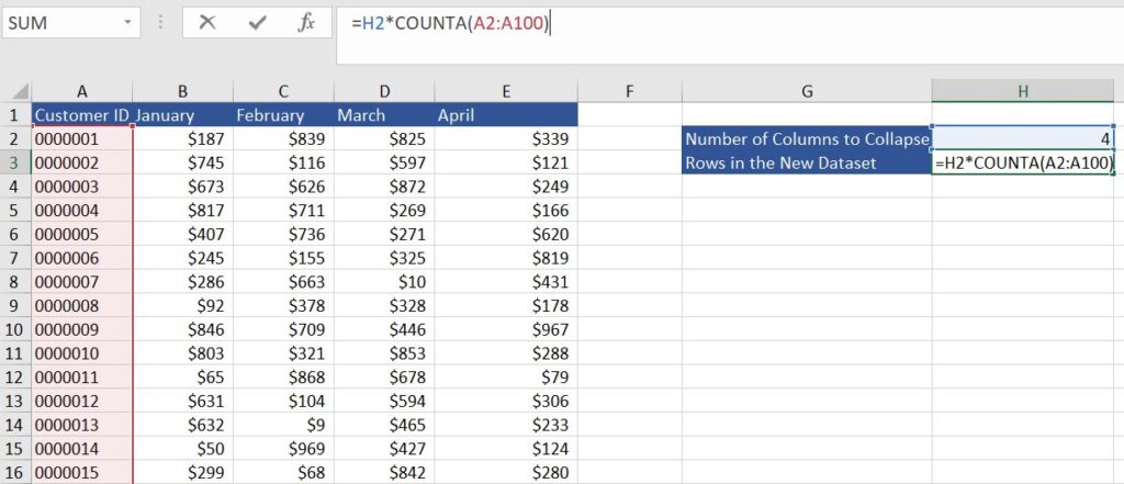
Step 1: Determine the Number of Columns to Collapse
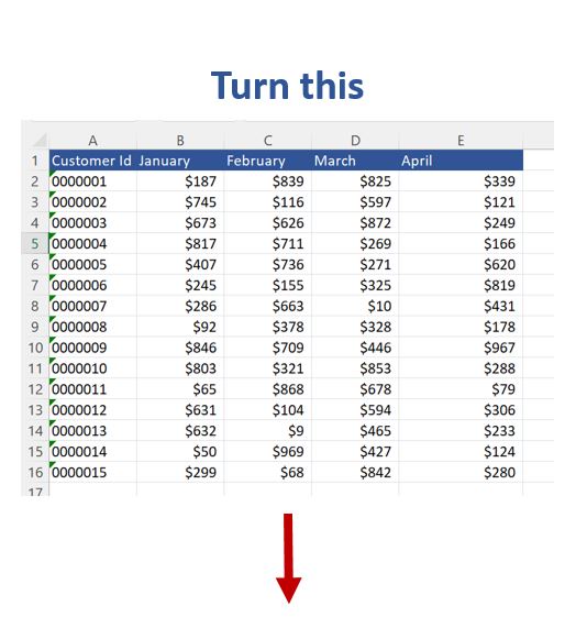
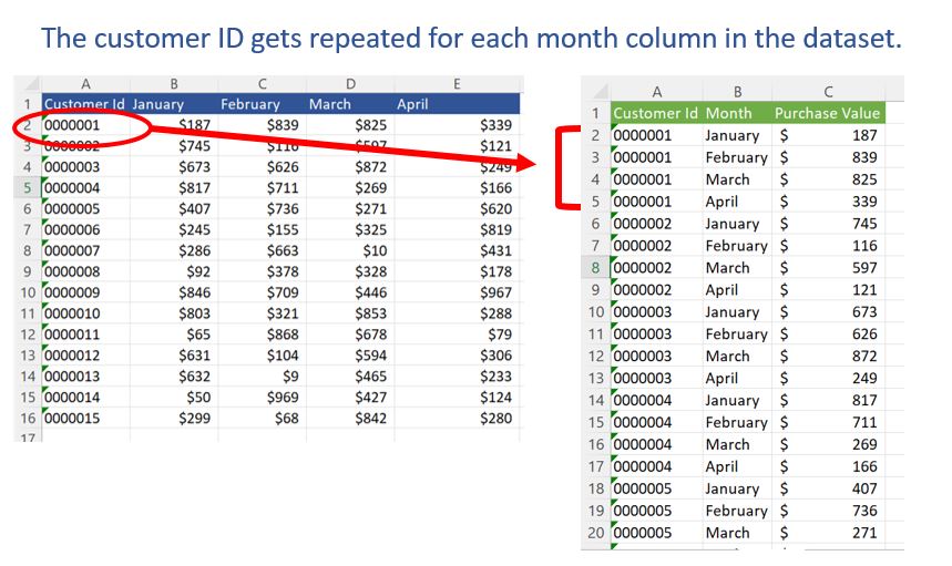
Let’s take the following customer purchases table as our example. When we “unpivot” the data, we really are repeating each customer ID for each column that we want to collapse.
We could simply type the number of columns we’d like to collapse in a cell, but let’s use a formula instead in case we ever want to make this a repeatable process. I like to use the COUNTA function starting at the first header and drag it to the right. COUNTA will count all the cells that aren’t blank (below, 4). If you update the data with new headers, the COUNTA function will then count those new headers.
Step 2: Determine the New Number of Rows of the Dataset
To determine the number of rows in the unpivoted dataset, we can multiply the number of columns we want to collapse by the number of rows in the current dataset. Again, use the COUNTA function and drag the formula down further than the current dataset to account for the dataset expanding in the future. This way, you don’t have to go back and change the formulas next time.
Step 3: Number your new rows to start creating the unpivoted table
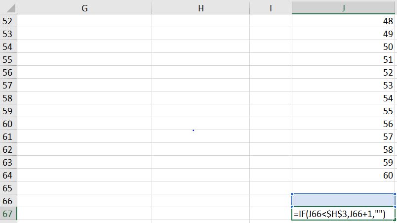
Write a formula to list numbers 1 through the total number of rows you calculated in Step 2. In this case, we are creating a formula to list the numbers 1 to 60. I like to set 1 as a value and then write a formula to add one to each cell until the value equals the max row value.
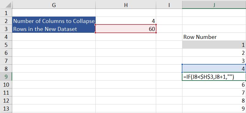
For a repeatable process, drag your formulas down further than the max row. The formula will already make any cell past the max row blank.
Step 4: Create a Cycle of Row Numbers from 1 to Your Header Amount that goes until the end of the new table
We need to repeat each Customer ID once for each column we are collapsing, which, in this case, is 4 times.
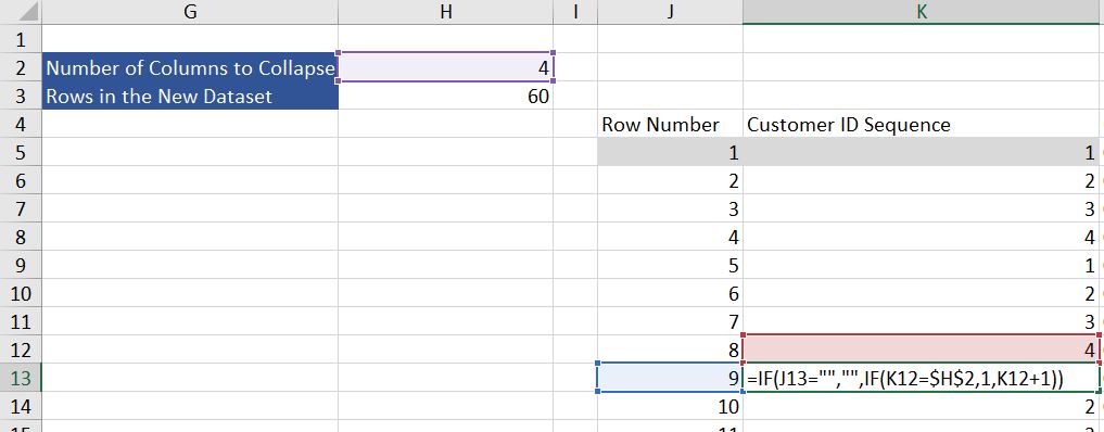
To account for a larger dataset in the future, add a quick if statement in the beginning that makes the cell blank if the row number is blank.
Step 5: Repeat the Customer ID Value Once for Each Number in Step 4
We now need to display the customer IDs next to the numbers we just created in Step 4. When the number in the Customer ID sequence switches from 4 to 1, we want to grab the next customer ID. To get the next customer ID, we will use an INDEX/MATCH function where the INDEX array is the customer ID column of the dataset. We will then find the Customer ID listed in the cell above in the original Customer ID column and add 1 to the MATCH, which will give us the next Customer ID in the list. Otherwise, if the number in the cycle is not 1 (in this case, 2 through 4), we set the formula to give us the Customer ID in the cell above the current cell.
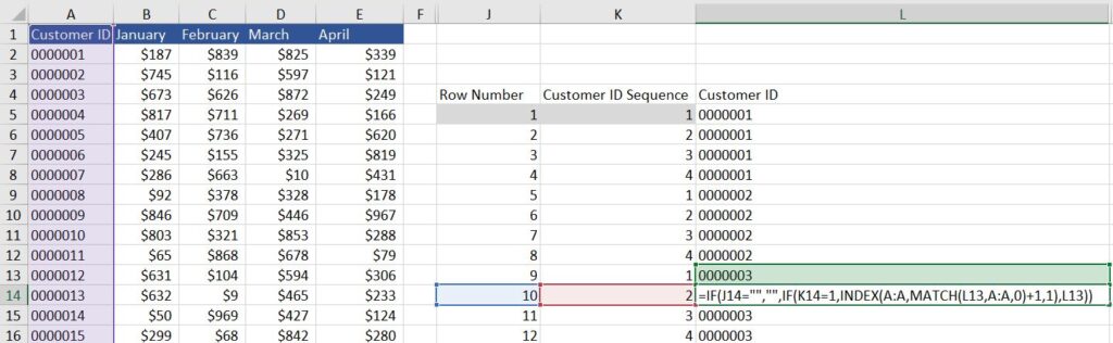
Some columns are hidden to make the formula easier to see.
Note: You must make the header column “Customer ID” the same name as the header name in the original dataset for this formula to work.
To make the process repeatable if the dataset grows, we add an IF statement at the beginning to set the cell value to blank if the row value is also blank. We can then drag the formulas below our current row values.
Step 6: List Each Month Once For Each Column ID
Now we need to add the collapsed column headers for each repeated Customer ID. All we need to do is use an INDEX where the array is the list of column headers (feel free to expand the length of your array to account for future column headers). The row number of the INDEX is 1 and the column number is equal to the Customer ID sequence.
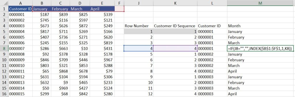
Just like in Step 5, to account for larger datasets in the future, we add an IF statement that sets the cell value to blank if the row value is blank
Step 7: Find the Sales Value Using the Customer ID and the Month
Finally, we can get the sales value for each Customer ID and Month by using an INDEX/MATCH function.
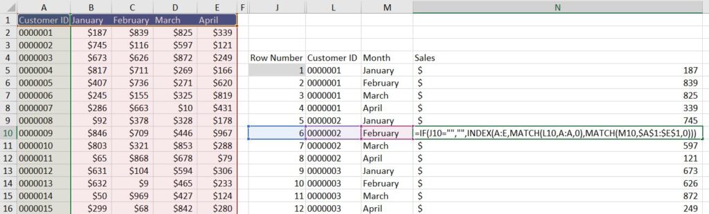
And we and an IF statement to account for an expanding dataset, just like in the other steps:
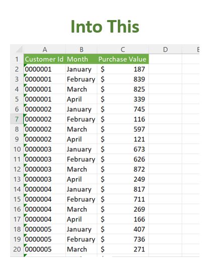
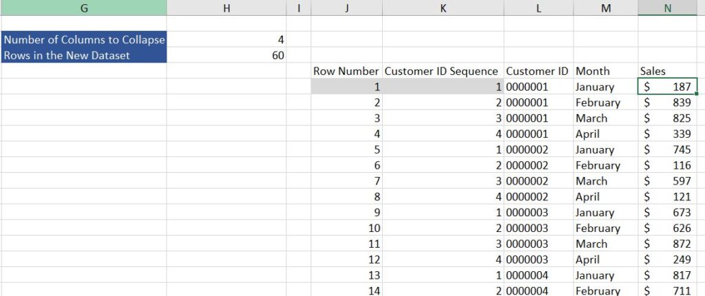
Conclusion – what your unpivoted data in Excel should look like after using formulas
And there you have it, your final dataset should look like this:
If you’re having trouble, or your situation is slightly different than the one above, feel free to email us at [email protected] for help! We also give free estimates for Excel work if you’d like to hire us for a larger project.