VLOOKUPs are one of the most widely used functions in Excel. They allow you to 1) extract specific data from a dataset or 2) join the columns of one dataset to another if they share some values in common.
While VLOOKUPs are useful and relatively easy to learn, they have two drawbacks:
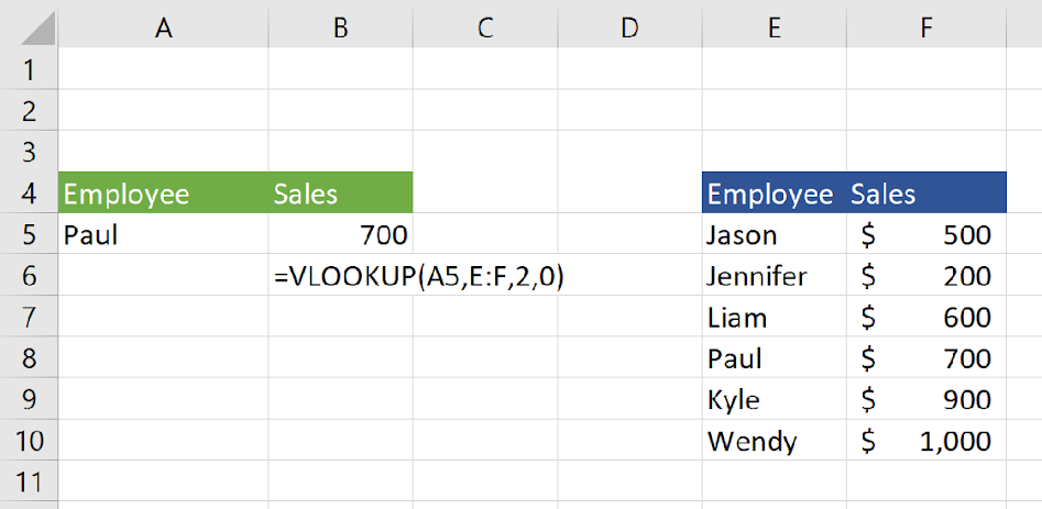
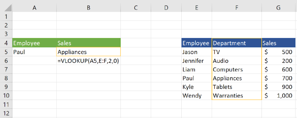
- If you use a static number for the column index, the formula won’t work if columns are inserted into the dataset or change order.
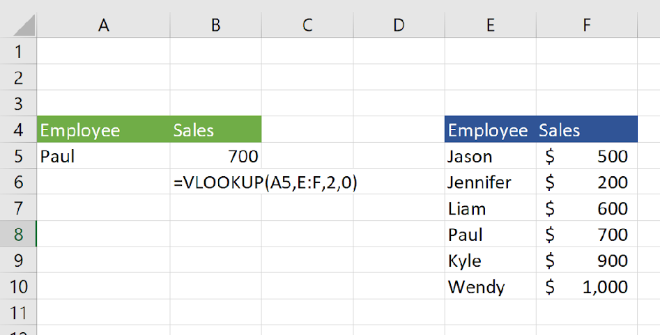
The VLOOKUP correctly pulls in sales for Paul in cell B5.
When we insert a column before Sales in the original table, the VLOOKUP now pulls in the Department value in cell B5 instead of Sales.

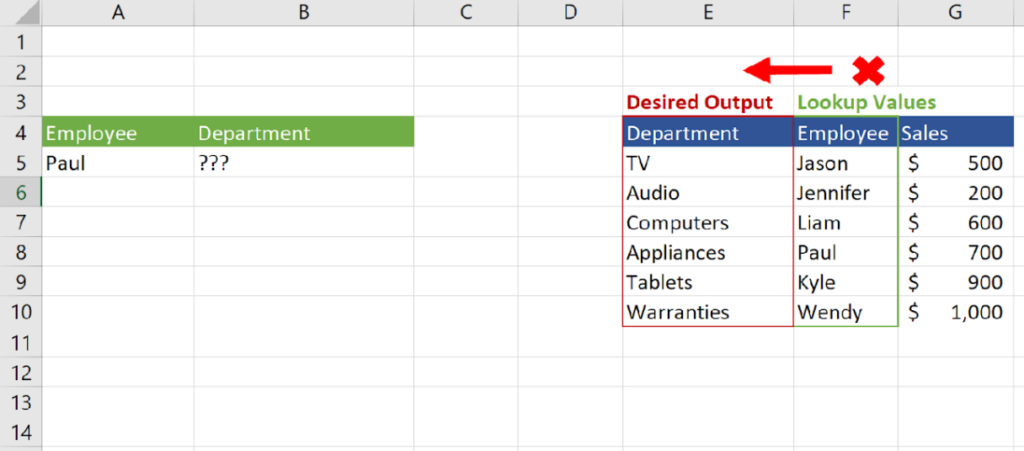
- The formula only works if your lookup values are to the left of the output you want to return in the table.
VLOOKUP can’t be used to lookup values in column F and return values in column E.
Let’s look at how to tackle each problem.
Making VLOOKUPs Resilient to Column Changes
MATCH
Adding a MATCH function for the column index of your VLOOKUP function can make the VLOOKUP dynamic—the function will still work if you add or change the order of columns in the dataset.
The MATCH function is rarely used on its own, but let’s review what the function does so that we can understand why it is useful in a VLOOKUP.
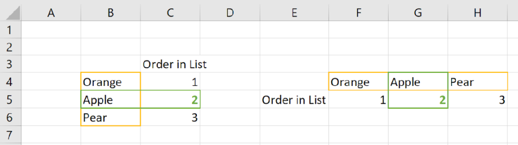
The MATCH function returns the numerical place of an input in a list. For example, if we search for the word “Apple” in the list below the MATCH function would return 2. The same is true if the list is organized horizontally.

Match Function Inputs:
MATCH(lookup_value,lookup_array, [match_type])
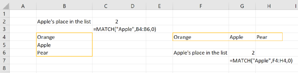
The MATCH function has three inputs. The first is the lookup value, or the value you want to search for in the list. In the example above, the lookup value is “Apple.”
The second input, called the lookup array, is the range of cells that make up the list you are searching in. Again, the list may be vertical or horizontal. In the prior example, the lookup array is B4:B6 for the vertical list, and F4:H4 for the horizontal list.
For now, don’t worry about the third input value, match_type. Always set that value to 0.
Therefore, a MATCH function for the example above would look like this:
VLOOKUP and MATCH
You can replace the column index of a VLOOKUP function with the MATCH function to make it dynamic. Let’s look at the example from before.
We used the number “2” to instruct the VLOOKUP to use the second column of the table for the output. Therefore, when we inserted a column before the Sales column, the VLOOKUP pulled the new column as the output since it was the second column in the table.
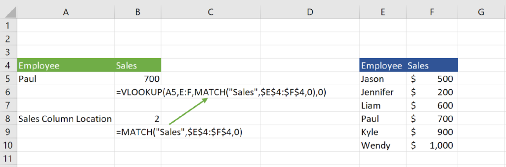
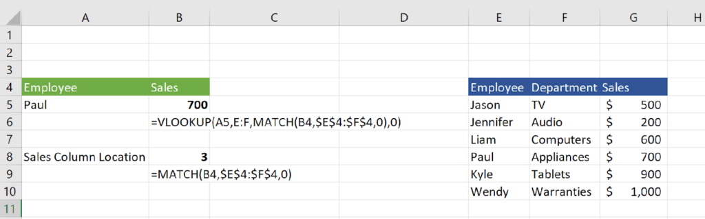
If we use the MATCH function, however, we can always have the VLOOKUP use the Sales column for the output, even if new columns are inserted into the table. Think of the column headers as a list, just like the list of fruit from the MATCH example above. The MATCH function can automatically tell us the location of the Sales column in the dataset:

Now we can insert the MATCH function into the column index portion of the VLOOKUP, and it will give us the same answer:
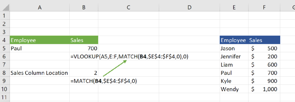
To make the formula a little cleaner, we can set the “Sales” part of the MATCH function to be equal to B4:
Now when we insert a column into the dataset, the VLOOKUP will adjust automatically and continue to pull in the Sales column as the output. Notice that the MATCH function now returns 3 instead of 2.
And there you have it: using the MATCH function with a VLOOKUP will make your VLOOKUPs resilient to inserted columns.
Look Ups That Go Right to Left:
The second problem with VLOOKUPs is that they only can look up values where the lookup value is on the left and the output is on the right.

Have no fear—Excel has a few functions that can serve this purpose.
INDEX/MATCH
Using the Index Function
A combination of the INDEX and MATCH functions can achieve a “right to left” lookup.
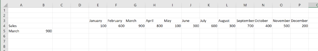
First, let’s review the INDEX function. The INDEX function returns the value of a cell in a table based on row and column inputs.
For example, the following formula returns 900 from the specified table.

Let’s look at the inputs:
INDEX(table_array, row_value, column_value)
The first input, table_array, is the range of cells forming the table you’d like to perform a lookup on. In the example above, the input is E4:F10.

The next input is the row_value. This input is the number of the row in the specified table of your desired output value. In the example above, the row_value input is 6.

The final input is the column_value. This input is the number of the column in the specified table of your desired output value. In the example above, the column_value is 2.
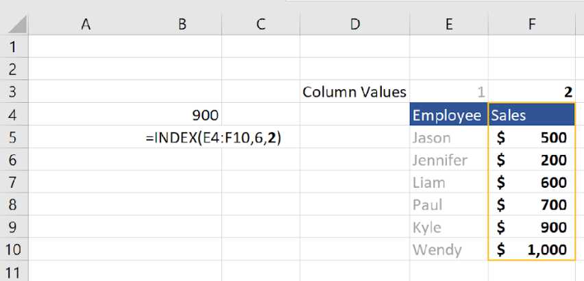
When row and column values are put together, they display the value in the 6th row and 2nd column of the table.

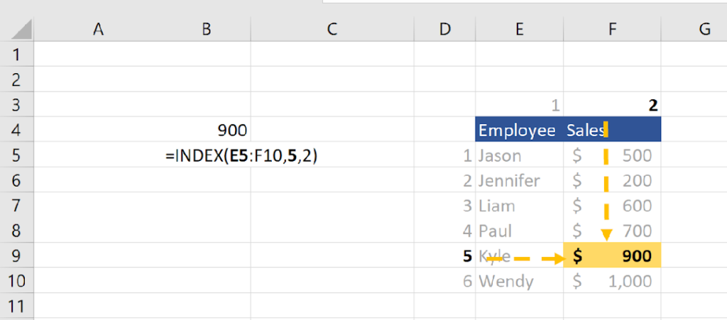
Note that the table range does not need to include the headers. If you decide not to include the headers in the formula, everything simply shifts down a row:
Using INDEX with MATCH
Much like using VLOOKUP with MATCH, adding MATCH functions to the INDEX function allows you to search for the row and columns for which you want to return an output value.
We can rewrite the example above with the row_value and column_value inputs being replaced by MATCH functions. Say we were looking for the “sales” made by “Kyle” in the table. An INDEX with MATCH functions can find the answer for us:

Right to Left Lookups with INDEX/MATCH
Unlike a VLOOKUP, an INDEX/MATCH can execute a lookup where the lookup value is to the right of the desired output value.
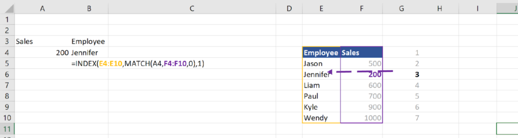
For example, say we wanted to see which employee had $200 of sales in the example table. We’d be unable to use a VLOOKUP function since the sales data, our lookup value, is located to the right of the employee data, our desired output. With an INDEX/MATCH function, however, we’d simply have to change the MATCH functions in the formula to find our answer.
In the previous example, we wanted the row value that corresponded with “Kyle” in the Employee column. In this case, we now want the row value where the Sales column is $200. Similarly, in the last example, our desired output was the Sales column. However, in this example we will switch the output column to the Employee column instead:
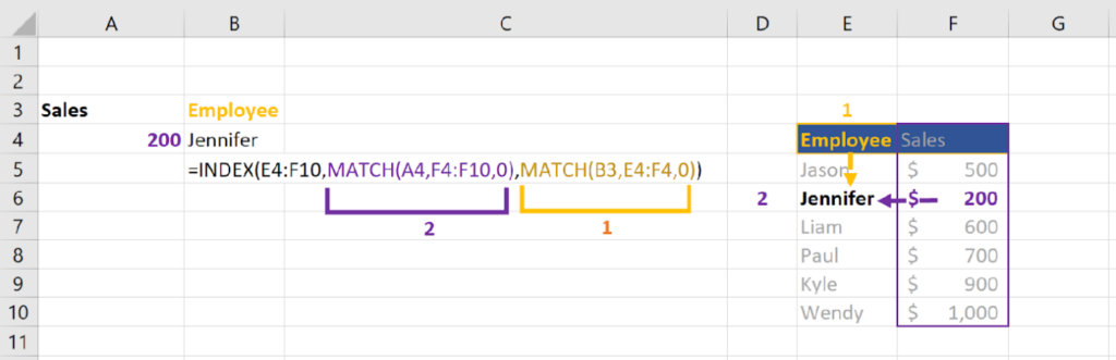
To sum it up: whether you are looking left to right or right to left, if you use and INDEX function paired with MATCH function, let the first MATCH function find the row of the lookup value in the lookup column. Then set the second MATCH function to find the column number of the title of the column that contains the value you are looking for, or the output value.
A Cleaner INDEX/MATCH
Analysts often to write the formula without a second MATCH. If you get confused at this part don’t worry. Just use the method described above. I wanted to include this section in case you see this variation in one of your spreadsheets.
The key difference with this method is that we don’t need to highlight the entire table for the first input in the INDEX function. Instead, we just need to highlight the column of our desired output value. Then we keep the MATCH in the row_values input the same and set the column value to 1. Let’s look at an example.
Recall the previous example where we trying to look up which employee had 200 sales in the table:

In this formula, we tell the INDEX function to look at the entire table, and we tell it exactly which row and column in that table to look at.
We can save ourselves a step if we just shrink the “table” input to just be the column that is going to contain the output value:

Now we just specify for which row in the Employee column we want an output value. In this case, it’s the row that “matches” the row in the Sales column that contains 200:

Then since there’s only one column in the table_input value, we can finish the INDEX function by typing a 1, instead of writing a second MATCH function:
For comparison, here’s the formula using the previous method. You can see the new formula is shorter.

Some people get confused because they incorrectly think the MATCH function must refer to data inside the table_input section of the INDEX formula. However, the formula still works even if the data looks like this:
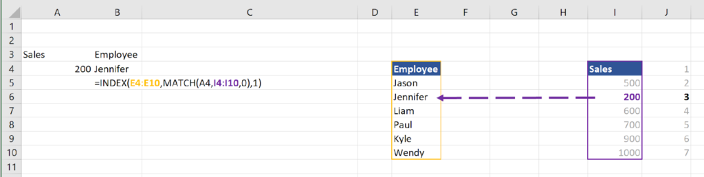
I explain this formula as:
=INDEX(answer_column, MATCH(lookup_value, lookup_column,0),1).
XLOOKUP
Microsoft realized the need to improve the lookup functions in Excel. VLOOKUP couldn’t look up right to left and its alternative, an INDEX function paired with MATCH functions, confused new users.
The solution: the XLOOKUP. XLOOKUP was rolled out in 2019, so you may not have it as an option if you do not have an updated version of Excel. The good news is that the XLOOKUP is very similar to the second version of the INDEX/MATCH formula–the inputs have just shifted around and it’s even easier.
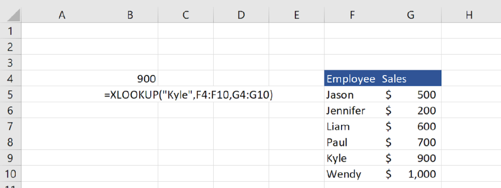
Here’s an example of the XLOOKUP in action:
Let’s check out the inputs:
XLOOKUP(lookup_value, lookup_array, return array)
The first input, lookup_value, is the input value you would like to match to in output value in another column. It’s the same as the lookup_value for a VLOOKUP. In this example, the lookup_value is “Kyle.”
The second input, lookup_array, is just a fancy way of saying “lookup_column.” The reason the input is called array is because the input can be a row or column, depending on which direction you are trying to go. For now though, think “lookup_column.” In this example, the lookup_array is “F4:F10.”
The final input, return array, is the column (or row) that has your desired output value. In this case, the return_array is G4:G10.
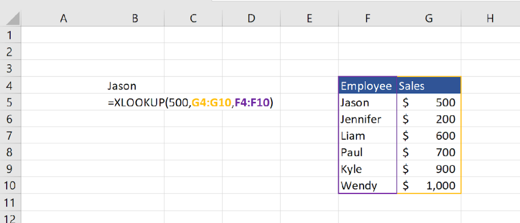
Like INDEX/MATCH, the XLOOKUP easily goes right to left:
It also goes up and down:
Conclusion
If you need to do a lookup function in Excel, use an XLOOKUP if you can. However, the other methods are still important to know because you’ll run across them in older spreadsheets. But remember, you don’t need to have your lookups messed up by inserted columns and you can perform a lookup in any direction you’d like.
Before you go: if you have any questions on this article or anything else Excel related, we are happy to help! Email us at [email protected] or check out our articles on improving a slow spreadsheet or alternatives to pivot tables.