Before we get started: If you have any questions on this article or anything else Excel-related, please email us at [email protected]! We also give free estimates for Excel work if you’d like to hire us. Or check out our article on improving slow spreadsheets.
Introduction to Pivots
Pivot tables are one of the most frequently used features of Excel. And it makes sense: they allow you to filter and analyze data in a user-friendly way. In fact, many people equate Excel proficiency with pivot table proficiency.
For one-off, exploratory analysis, pivots work well. But if you are creating a workbook that will be updated regularly, I’d recommend replacing the pivot tables with formulas, especially if the pivot is in the middle of your process rather than the end product.
The Downsides of Pivots
Pivot tables have a few drawbacks for frequently updated files:
1) You must remember to update them
That sounds like an easy task, but I can’t tell you how many times I’ve spent an hour analyzing a file with my team only to realize we never refreshed a pivot. And that’s for a team of experienced Excel users—imagine if you were creating a file for a non-experienced client to use. The problem happens often when the pivot is on a different tab than the data input since there’s no visual cue to remind the user to update the pivot table.
It’s possible to refresh a pivot automatically when opening a workbook, but that’s not helpful for frequently used files. Typically, I open files to add new data, which requires me to refresh the pivot again once the data is added.
2) A filtered pivot excludes new categories by default
Say you create a pivot table with a filter:
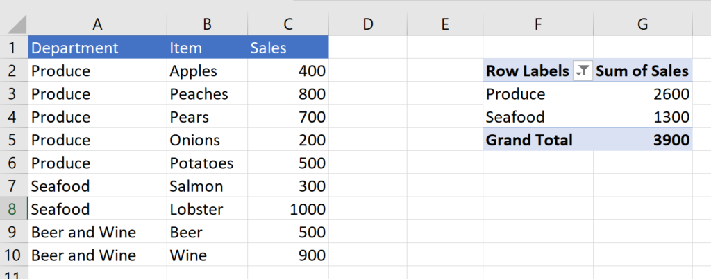
You then filter out the “Beer and Wine” category because you don’t want to include any beverages in your analysis.
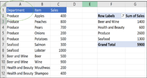
The next time you open the file, you add more data, but the new category is excluded:
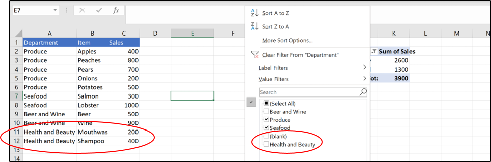
The Health and Beauty category doesn’t pull into the pivot.
Although this is a simple example, the problem becomes worse when the dataset includes thousands of rows with many categories. It’s easy to miss that a new category has appeared in the data and isn’t being added to the pivot. Then that data unwittingly gets excluded from the rest of the model.
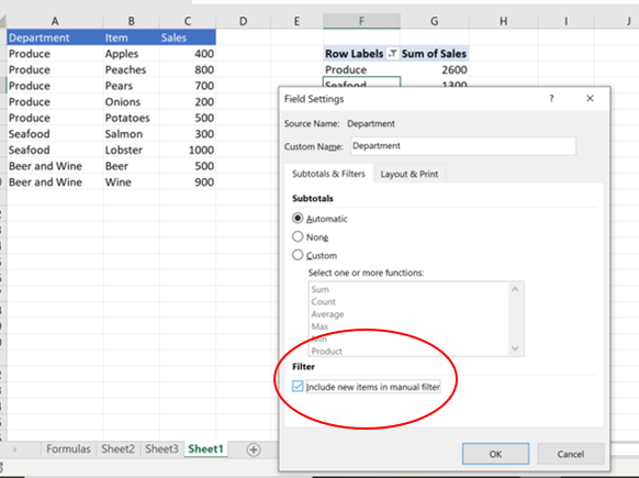
It is possible to change the pivot’s settings to combat the problem: right click the pivot, select field settings, and then click “include new items in the manual filter.” Still, I think it’s safer to avoid the issue altogether.
3) Pivots break when a header changes
When the header in column A changes from “Department” to “Section,” the pivot table drops its row labels.
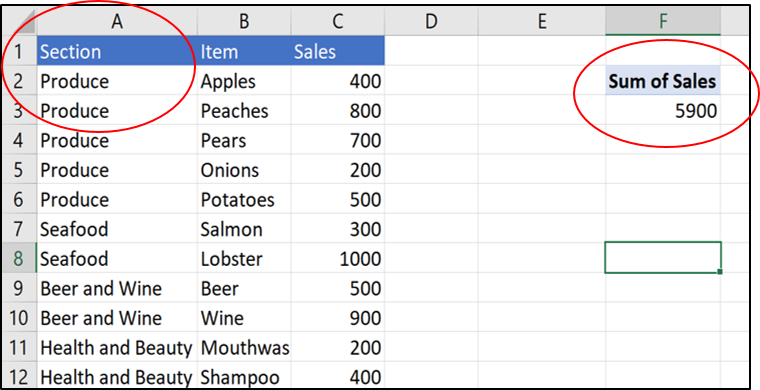
It’s easy to imagine a client or another analyst updating the header title without realizing that they’re breaking a pivot used later on in the process. Or, the pivot will break if the headers of the dataset change in the original data source. Again, when a dataset contains dozens of columns, it’s easy to miss when a single header changes.
Consider Using Formulas
Luckily, you only need to use a few formulas to replicate a pivot table, and the new table created by formulas will automatically expand and change when the underlying dataset changes.
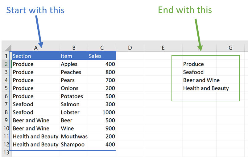
The main advantage of a pivot is that it quickly identifies unique values in a column – i.e., the pivot reproduces the column without duplicates—and then summarizes the data by those unique values. In the example above, the pivot aggregates the values in column C for each of the categories listed in column A (Produce, Seafood, Beer and Wine, and Health and Beauty).
The goal of the formulas should be the same: to identify the unique values in a column and reproduce them in a separate table every time the data is updated. Then we can use formulas that reference the unique list to summarize the data.
I’ve used two methods to accomplish this task.
The Sorting Method
If you can sort the data by the categories you are trying to identify, it’s easier to create the list of unique values.
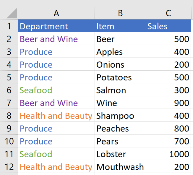
Let’s use the same example as before. I sorted the data this time.
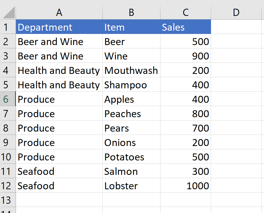
Our goal is to tag each new department name the first time it appears, but not again afterward. Because the data is sorted, we can create a tag each time the values change in column A.
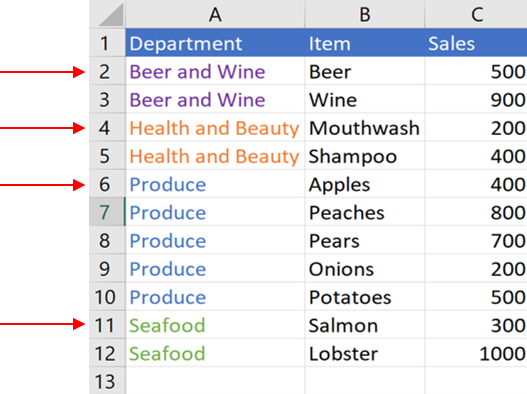
Here’s an example of a formula to create the tag:
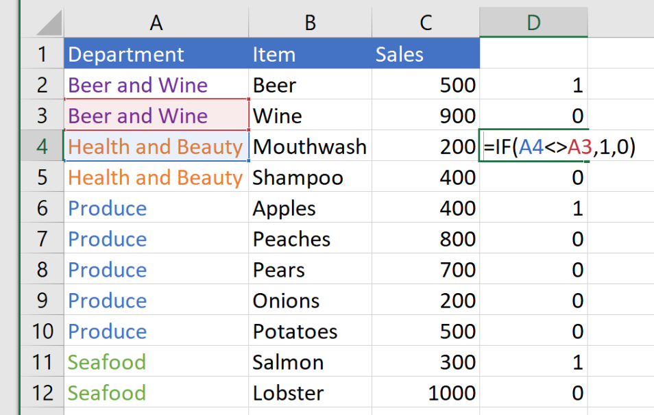
In short, the formula says that if the cell in the current row is not equal to the cell above it, put a 1; otherwise, put a 0. If we could pull all the values in column A where the value in column D is 1, then we would have our list.
The problem is that, currently, all the values we want to pull in column A are represented by the same 1 value in column D. So an XLOOKUP off of column D using 1 as the match value would keep giving us “Beer and Wine” since it appears first in the list.
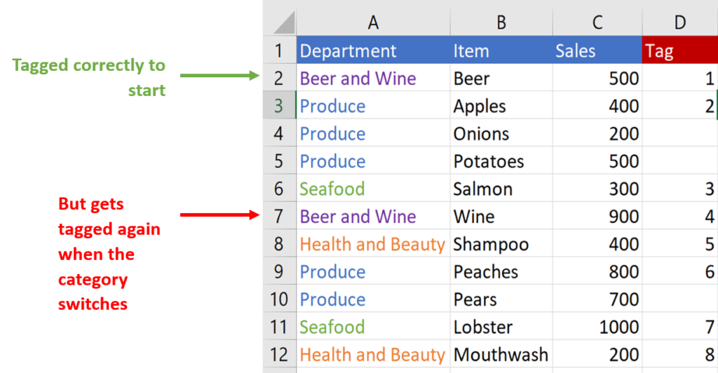
Instead, we have to distinguish between each 1 value. I like to incrementally increase the values, so the first tag is 1, the second is 2, and so on.
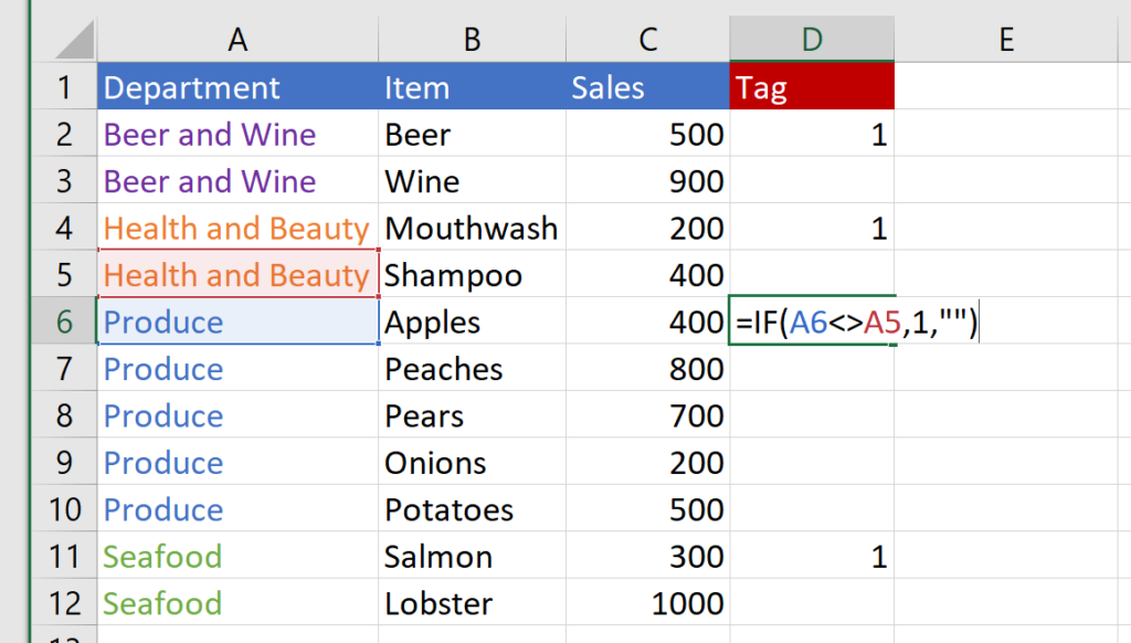
And to make it cleaner and assist the formula, I’ll also change the 0 values to blanks instead:
Step 1—Change the 0s to blanks. To create blanks, use “” in your formula:
Step 2—Where the 1 is currently located in the formula, put a COUNT function instead. Lock the start of the COUNT functions range as $D$1 and set the end of the range to the cell above the formula, unlocked. Then add +1 to the end of that formula.
Here’s the example:
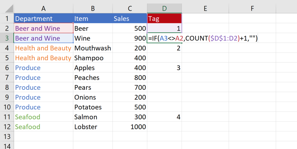
The function checks to see if the value in column A has changed compared to the cell above it. If it has, it then sees how many number labels are above the current cell in column D and adds one.
The result is that every time a new value appears in column A, the formula will assign it a unique number.
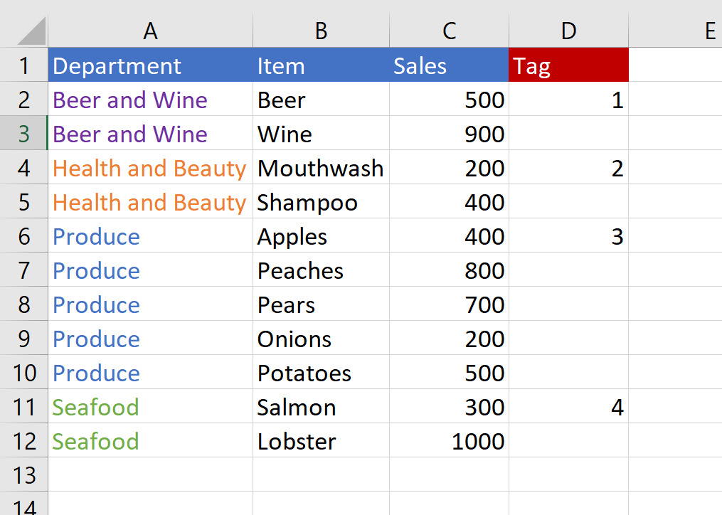
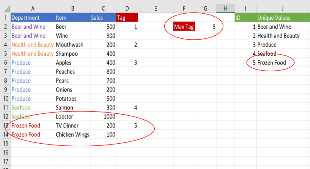
The next step is to write the numbers somewhere else in the sheet, and then pull the unique values in column A using the numbers in column D as lookup values.
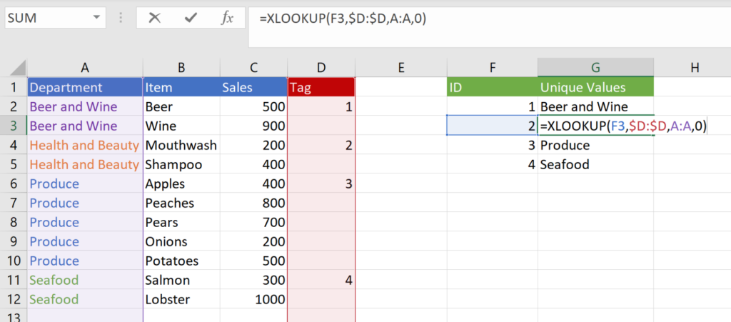
Instead of typing the values directly into column F, we can use formulas. That way, if the number of tags increases, the ID list in column F will increase as well.
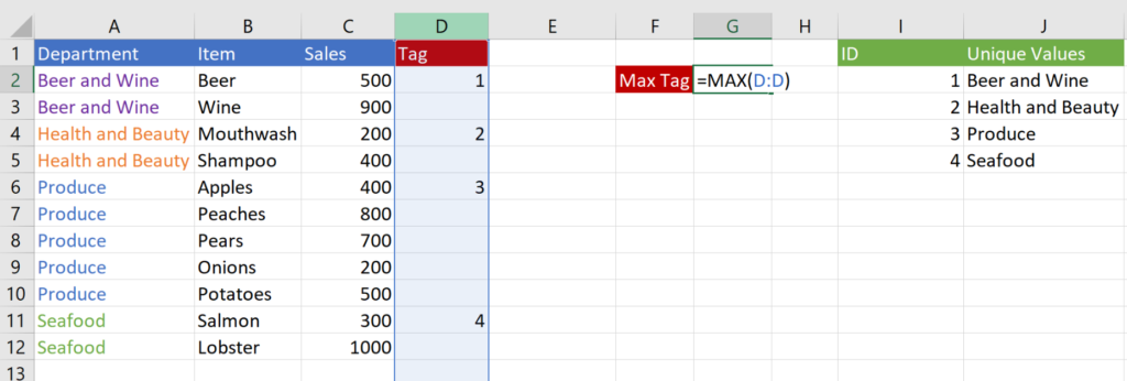
Step 1—Write a formula that will calculate the max value in column D:
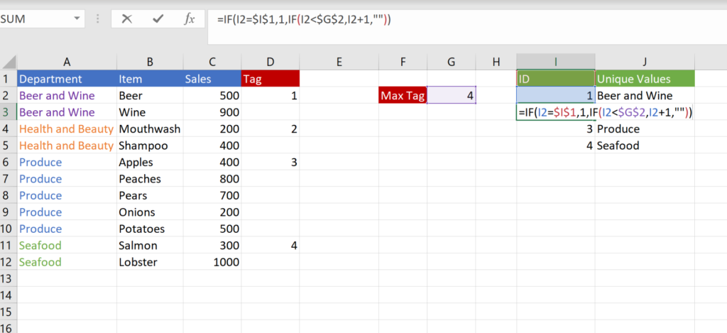
Step 2—In column I, set each cell to be one number greater than the value above it as long as the number above it is less than the max number. (Since there isn’t a number above cell I2, I usually write a quick IF statement to say if the cell above is equal to the title of the column, then make it 1).
Now that the formulas are all set up and working, we need to drag down the formulas in columns D, I, and J to account for new data being pasted in. We can set those formulas to return a blank value if there is no data in the same row. If data is pasted into that row, however, the formula will then determine if a new tag must be added. Depending on the dataset and how much it changes, I like to drag the formulas at least 10% past the last row of the current data.
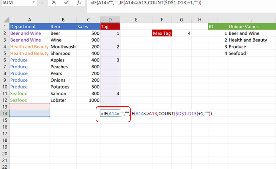
The red outline shows what we added to the formula to set it to blank if there isn’t any data in the row. The formula in column I can be dragged down as is. However, add the same code to column J that makes the formula blank if column I is blank and drag it down 5-10 rows past the current values in column I.
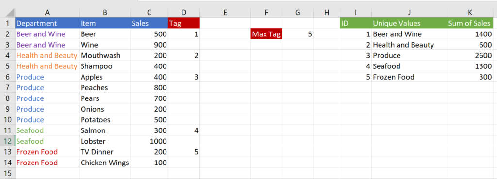
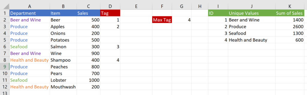
Now look what happens when we add a new category to the underlying data in columns A:C:
The tag formulas create a new tag, 5, in column D for the new Frozen Food category. The max formula then adjusts to 5, which causes the ID formula to create a new 5th row in the table. And it all happened automatically.
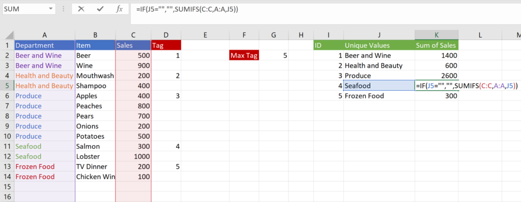
Finally, use a formula in column K to summarize the data by category, just like you would in a pivot. Don’t forget to drag the formula down a few extra rows and set it to be blank if the data in column J is blank.
And there you have it—so long as the formulas in D, I, J, and K are dragged down far enough, you’ll never have to worry about refreshing the table again.
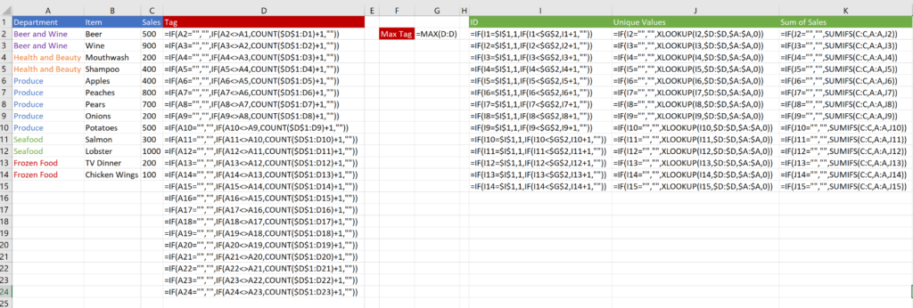
Here’s what it all looks like in formulas:
If the data isn’t sorted
If you can’t sort your input data before it goes into the Excel Workbook, that’s okay. You’ll just have to adjust the formula in column D to account for the fact that the categories will be all over the place. Everything else will work the same.
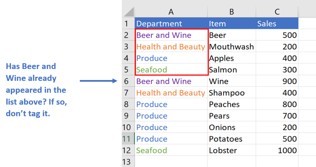
Let’s look at the table again when it is unsorted:
Unlike when the table is sorted, we can no longer identify unique values by checking if the cell above the current cell is a different value. Otherwise, our tag will tag the same category multiple times:
What we need to do now is check if the value has already appeared anywhere above the cell in column A. Then we can tag the first instance of each category.
To accomplish this, we just have to adjust the part of the tag formula that checks if the cell above is equal to the value of the cell in the same row of column A.
As a reminder, here is what the formula looked like when the data was sorted last time:
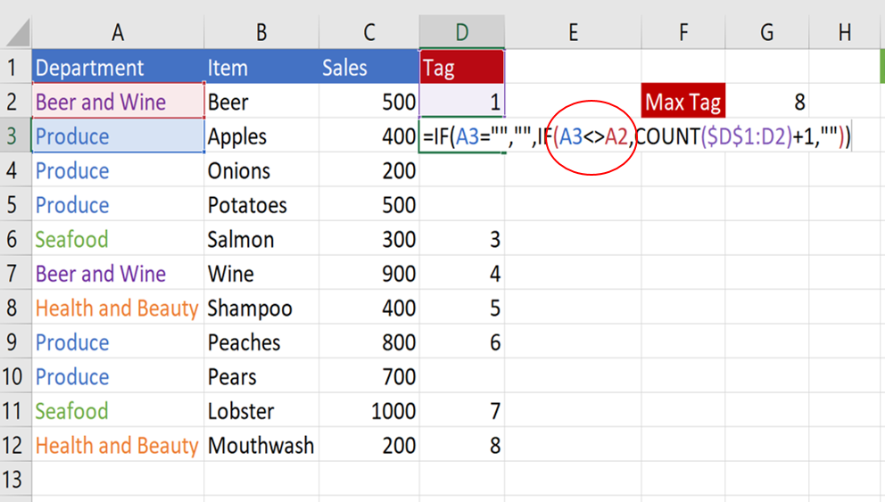
We need to change the part of the formula highlighted by the red circle. Delete the A3<>A2 section of the formula and replace it with the COUNTIF shown below:
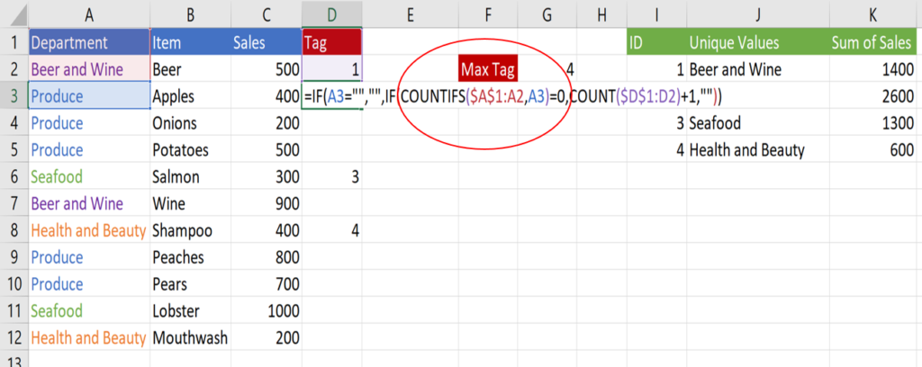
The COUNTIFS function looks at the value in the same row in column A and checks if that value has appeared anywhere in the column above the current row. Just like the COUNT function later on in the formula, the start of the range is locked, while the end of the range is unlocked so that the range expands as the formula is dragged down.
And that’s it.
In general, this formula is slower than the formula used when the data is sorted, but the speed should be negligible unless the file is large.
Conclusion
For a frequently updated file, you should seek to eliminate as many steps by the user as possible to reduce the chances of error. Although pivots are a tempting tool to use as part of a process within an Excel file, they can increase the chance of a user making a mistake. You can replace the pivots with formulas to eliminate these problems if the file can support the extra computing power needed to execute the formulas.
If you’re looking for extra help to make your spreadsheets better, check out our article on improving slow spreadsheets or email us at [email protected]!