A VLOOKUP is one of the most common functions in Excel. It allows you to “look up” a value in a table and return the corresponding value of another column.

One of the trickiest parts of a VLOOKUP, however, is understanding what to put as the column index number.

Remember, a VLOOKUP function looks up a value in the leftmost column of a table and returns the corresponding value in another column of the same table. The column index number simply tells Excel from which column in the table you’d like to return a corresponding value. That “corresponding value” column is represented by the number, counting from left to right, of the column in the table.
How to Know the Column Index Number in a VLOOKUP
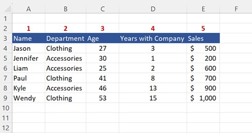
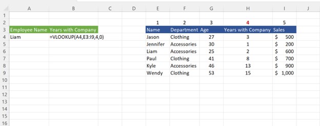
Check out the table below.
If you used a VLOOKUP that took “Name” as a lookup value and highlighted the blue table as the table input for the function, you could then choose any of the numbers from 1-5 for the column index number to return a corresponding value for the name you are looking up.
For example, a column index number of 3 returns the employee’s age, while one of 5 returns the employee’s sales.
Examples of Using the Column Index Number in a VLOOKUP
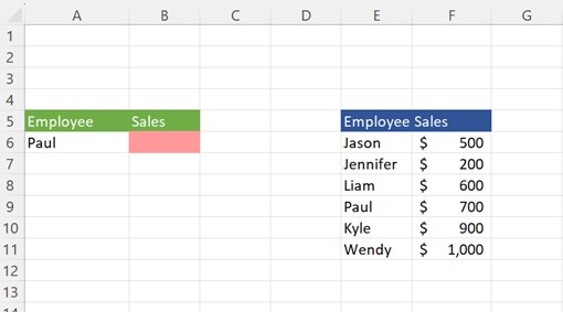
Let’s take a look at our original example.
We’d like to find the dollar amount of sales generated by the employee Paul using the blue sales table. We want the answer to appear in cell B6.
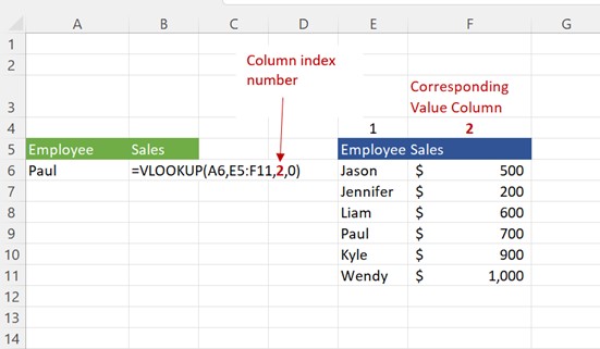
In our VLOOKUP function, the “lookup” value is A6 (“Paul”), the table input is E5:F11 (the table in blue), and the column index is 2 because “Sales” is the second column in the table we’ve highlighted.
Now let’s look at an example using a different table. Say we wanted to find the number of years Liam has been part of the company. Which column index number would we use if the input table is E3:I9?
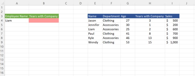
We’d input a column index number of 4 since “Years with Company” is the 4th column in the table:
Column Index Number when the VLOOKUP Starts in the Middle of the Table
The table input of a VLOOKUP function doesn’t need to start at the beginning of a table. Let’s say we switched the order of the department and name columns in the previous example.
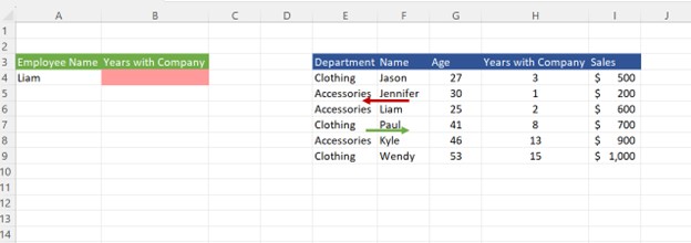
Because we’d still like to look up Liam’s years with the company, we must define our table input for the VLOOKUP with “Name” as the first column of the table.
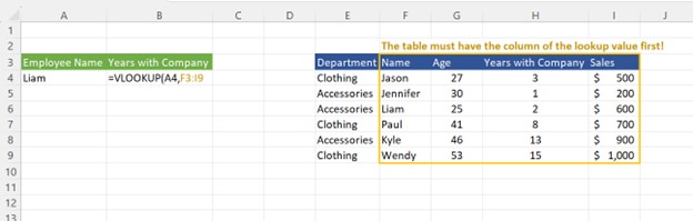
The column index number is the column number of the user-defined table, not the entire blue table overall.
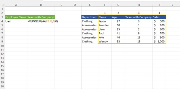
Because the input table in the function starts in column F and not column E, the column index number for “Years with Company” is now 3 instead of 4.
Conclusion and Issues with VLOOKUPS
In many professional spreadsheets, you’ll rarely see the column index number expressed as a standalone number typed into a formula. Instead, you’ll likely see a MATCH function in the column index number’s position in the function.
Why?
If a column is inserted into the lookup table it can change the column index number for the answer column. For example, I inserted a “Gender” column into the table below, which now changes the proper column index number for “Years with Company” from 4 to 5:
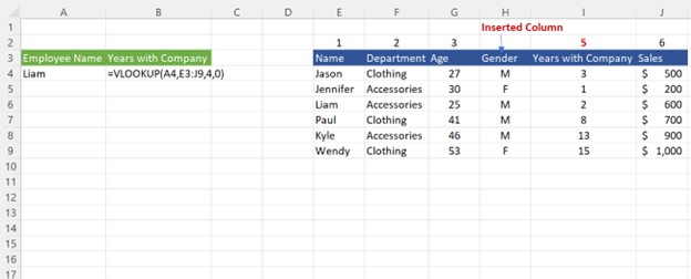
As a result of the inserted column, the VLOOKUP would incorrectly show Liam’s gender instead of his Years of Service.
To avoid such problems, many analysts choose to write a MATCH function to dynamically select the column index number instead of typing the number into the VLOOKUP function directly or use other lookup functions entirely.
But by grasping the basics of a column index number, you can use VLOOKUP functions properly and understand the foundations for advanced Excel techniques.